How to Use Sumif Functionality in Excel?

In Excel, we often have multiple dimensional dataset wherein there are more than 1 attribute of the data and corresponding to it, we have certain numerical values.

Lets see an example of such a dataset below. Look at the data carefully.

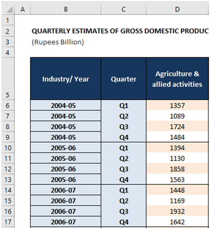
In the above dataset, we have the year labels in column B, the quarter labels in column C and the value of the Agriculture & Allied Activities sector in column D.

So there are 2 main attributes in the above dataset i.e. Years and Quarters. And against each of those two attributes we have the GDP contribution value of the Agriculture and Allied Activities sector.

Clear so far? Good.

Now, let us say, we want to calculate for any given year, what is the total of the quarterly values for Agriculture sector?

So if the user wants to calculate for the year 2004-05, the total of Agriculture sector values are=SUM(D6:D9) i.e sum of (1357+1089+1724+1484) = 5654.

And for the year 2005-06, the total would be=SUM(D10:D13), i.e. sum of (1394+1130+1858+1563) = 5945.

This is pretty straight forward isn’t it? Yes, it is.

If you notice carefully, we are adding up the different values corresponding to the particular year only. That is we are making a conditional SUM such that it only adds up those years where the year matches the desired value i.e. 2004-05 or 2005-06 or 2006-07.

This is where the SUMIF function comes in handy in Excel. It allows us to write a formula in one single shot that can add up only those values where a certain condition is met. In this case, we want to add up the Agriculture and Allied Activities sector values corresponding to a certain year only.

Let us see how we can do that. Given any specific year, how do we write the SUMIF formula to get the total of the Agriclture and allied activities sector value.

SUMIF SYNTAX

The SUMIF function requires the following three elements as part of its syntax:

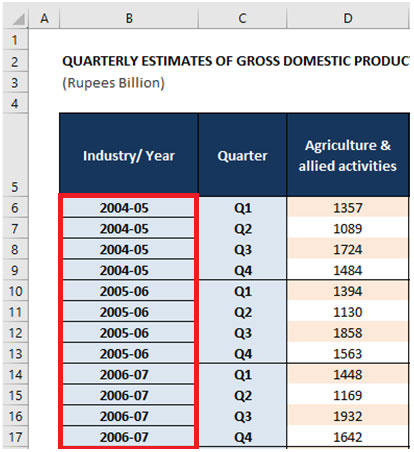
1. Range: The range of cells on the sheet that corresponds to the respective condition dimension. Like in our above example, we want to add up the values corresponding to the year dimension. So we need to specify the entire range of values where the year data is mentioned. In case of the above dataset, the range would be cells B6:B17 (see the red colored box)

 

2. Criteria: In the provided range of cells, what is the specific condition that needs to be met. That is the criteria of the SUMIF function syntax. In the above, let us say, we want to do this for the year “2006-07”?So the criteria would be the value “2006-07”. You can provide this as a text value inside the formula or also link it to a cell that contain this value.

 

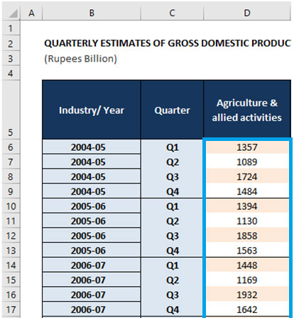
3. SumRange: This is the range of all the cells that contain the values to be added up. In our above example, we need to specify the cells D6:D17as it is the range of all the cells that will need to be added up corresponding to the criteria.

So, the final formula will become = SUMIF(RANGE,CRITERIA,[SUMRANGE])

For the example, we are working on if we want to find out the value for the year “2006-07”, then we write it as = SUMIF (B6:B17, “2006-07”, D6:D17)

This formula will add up the values for the year 2006-07 in the entire range of Agriculture and allied sector values, i.e = (1448+1169+1932+1642) = 6192 as the result of the same.

[Aside] If you want the results for any year, just mention it within quotation marks i.e. “2004-05” or “2005-06” or “2006-07” etc in the criteria portion of the formula. It will accordingly add up values meeting that particular criterion only.

 

IMPORTANT THINGS TO REMEMBER ABOUT SUMIF FUNCTIONALITY IN EXCEL

Now, while the formula is pretty straightforward, it requires a bit of practice at your end as well. In our experience, there are a few IMPORTANT thingsto make note of while writing this formula for our real work. Some of them are as follows which we should remember:

1. The Range is different from SumRange – While they sound similar, they are pretty different from each other. The Range refers to the values that will meet the criteria and the SumRange is the values which we need to add up subject to the criteria being met.

 

2. Range comes before SumRange : In the formula syntax, the Range is the first part of the syntax followed by the Criteria and then followed by the Sum Range. Often, we can confuse it to be opposite which will lead to a wrong result. So we need to be careful about that.

 

3. Criteria can be in a different cell: In our above formula, we have put the criteria inside the formula i.e. “2006-07”. In practice, we can also put the criteria in a different cell and reference the particular cell in the formula. Let us say in our above formula we can reference it as cell B14 which contains the value “2006-07”. In general, it is a good idea to put values in a cell and then reference it in the formula.

 

4. Criteria can also contain “>” or “<” or “<>” conditions: Let us say in our above formula, we wanted to add up all the Agriculture and allied activities value for all years except “2004-05”. In that case, we can change the criteria value to be =“<>2004-05”. The <> sign represents not equal to and will add up all those values for which the years are not 2004-05. It is a very useful variation of the SUMIF formula that can help us to add more conditions in the criteria to provide more useful calculations on a dataset.

 

So as you can see, the SUMIF functionality can be very useful for finding conditional totals in a dataset. As long as there is one condition to be met, the SUMIF is a great resource to use. Check it out yourself.